5. PM4NGS for RNA-Seq data analysis

Differential expression (DE) analysis allows the comparison of RNA expression levels between multiple conditions.

The differential gene expression and GO enrichment pipeline is comprised of five steps, shown in next Table. The first step involves downloading samples from the NCBI SRA database, if necessary, or executing the pre-processing quality control tools on local samples. Subsequently, sample trimming, alignment, and quantification processes are executed. Once all samples are processed, groups of differentially expressed genes are identified per condition, using DESeq and EdgeR. Over- and under-expressed genes are reported by each program, and the interception of their results is computed.

Finally, once differentially expressed genes are identified, a GO enrichment analysis is executed to provide key biological processes, molecular functions, and cellular components for identified genes.

DGA and Go enrichment, RNASeq pipeline

Step	Jupyter Notebook	Workflow CWL	Tool	Input	Output	CWL Tool
Sample Download and Quality Control	Pre-processing QC	download_quality_control.cwl	SRA-Tools	SRA accession	Fastq	fastq-dump.cwl
			FastQC	Fastq	FastQC HTML and Zip	fastqc.cwl
Trimming	Samples trimming		Trimmomatic	Fastq	Fastq	trimmomatic-PE.cwl trimmomatic-SE.cwl
Alignments and Quantification	Alignment and Quantification	rnaseq-alignment-quantification.cwl	STAR	Fastq	BAM	star.cwl
			Samtools	SAM	BAM Sorted BAM BAM index BAM stats BAM flagstats	samtools-view.cwl samtools-sort.cwl samtools-index.cwl samtools-stats.cwl samtools-flagstat.cwl
			IGVtools	Sorted BAM	TDF	igvtools-count.cw
			RSeQC	Sorted BAM	Alignment quality control (TXT and PDF)	rseqc-bam_stat.cwl rseqc-infer_experiment.cwl rseqc-junction_annotation.cwl rseqc-junction_saturation.cwl rseqc-read_distribution.cwl rseqc-read_quality.cwl
			TPMCalculator	Sorted BAM	Read counts (TSV) TPM values (TSV)	tpmcalculator.cwl
Differential Gene Analysis	Differential Gene Expression Analysis		DeSEq2	Read Matrix	TSV	deseq2-2conditions.cwl
			EdgeR	Read Matrix	TSV	edgeR-2conditions.cwl
Go enrichment	Gene Ontology Enrichment		goenrichment	gene IDs	TSV	Python code in the notebook

5.1. Sample sheet

Sample Sheet for Drosophila BioProject PRJDB5673

sample_name	file	description	replicate	condition
DRR092341		Wild type, adult male head, replicate 1	1	WTAdult
DRR092342		Wild type, adult male head, replicate 2	2	WTAdult
DRR092343		Lol mutant, adult male head, replicate 1	1	LolAdult
DRR092344		Lol mutant, adult male head, replicate 2	2	LolAdult

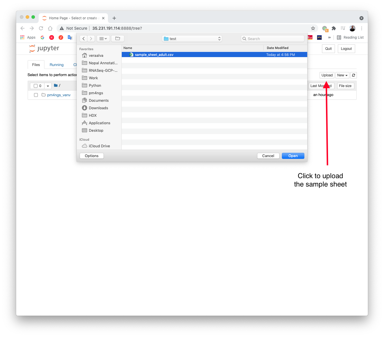
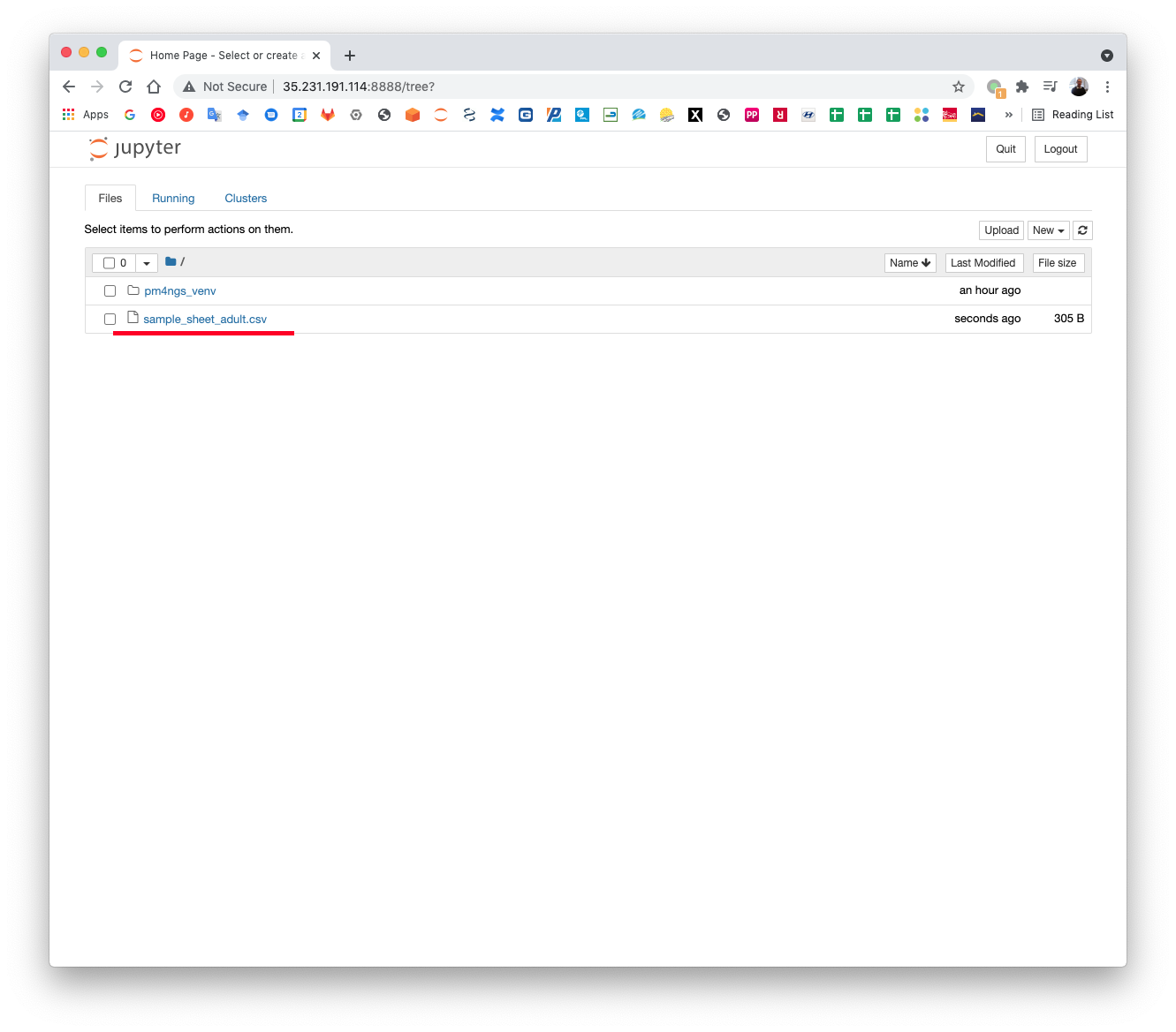
Download the sample sheet file to your local computer: sample_sheet_adult.csv

Upload the sample sheet file to the GCP instance through the Jupyter server

5.2. Creating the PM4NGS RNA-Seq project

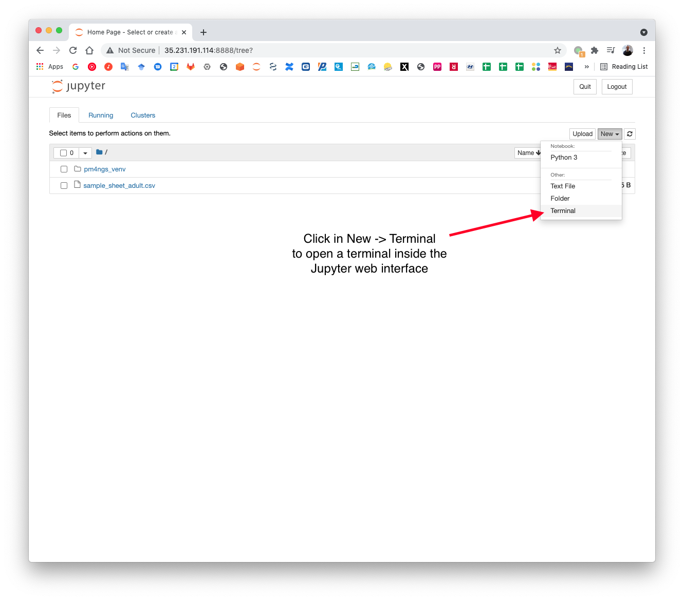
Open a terminal to execute pm4ngs-rnaseq. This command will create an organizational data structure for the analysis.

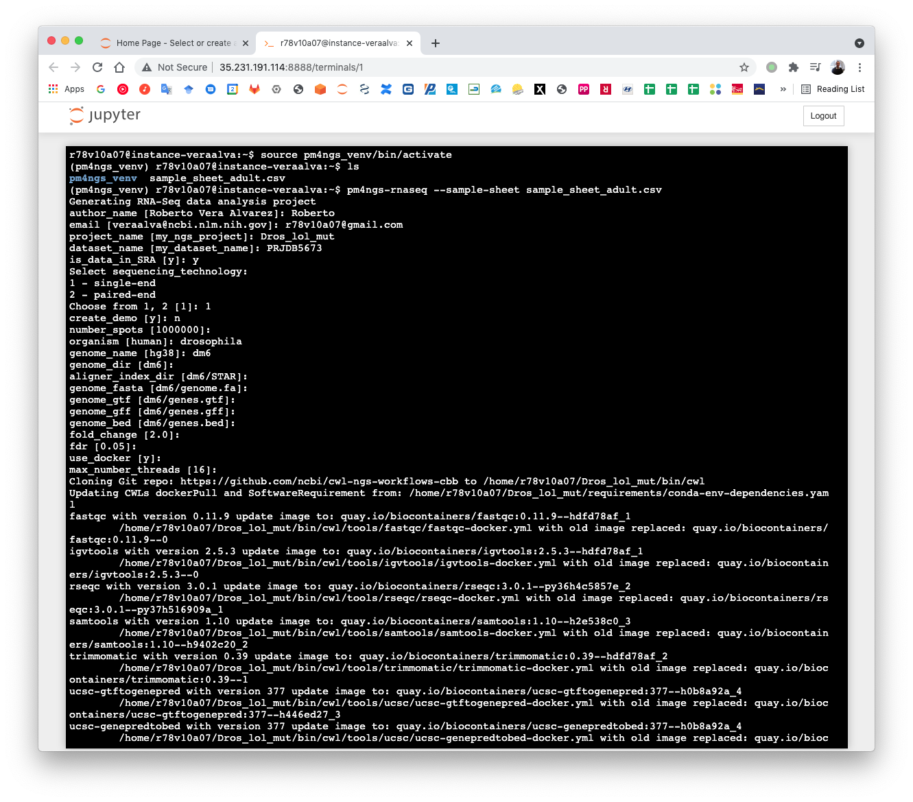
In the terminal, activate the pm4ngs_venv virtual environment and execute the pm4ngs-rnaseq command.

The pm4ngs-rnaseq command line executed with the --sample-sheet option will let you type the different variables required for creating and configuring the project. The default value for each variable is shown in the brackets. After all questions are answered, the CWL workflow files will be cloned from the github repo ncbi/cwl-ngs-workflows-cbb to the folder bin/cwl.

r78v10a07@instance-veraalva:~$ source pm4ngs_venv/bin/activate
(pm4ngs_venv) r78v10a07@instance-veraalva:~$ ls
pm4ngs_venv  sample_sheet_adult.csv
(pm4ngs_venv) r78v10a07@instance-veraalva:~$ pm4ngs-rnaseq --sample-sheet sample_sheet_adult.csv

Note

• author_name:

  Use your full name

• email:

  Use your email

• project_name:

  Name of the project with no space nor especial characters. This will be used as project folder's name.

  Use: Dros_lol_mut

• dataset_name:

  Dataset to process name with no space nor especial characters. This will be used as folder name to group the data. This folder will be created under the data/{{dataset_name}} and results/{{dataset_name}}.

  Use: PRJDB5673

• is_data_in_SRA:

  If the data is in the SRA set this to y. A CWL workflow to download the data from the SRA database to the folder data/{{dataset_name}} and execute FastQC on it will be included in the 01 - Pre-processing QC.ipynb notebook.

  Set this option to n, if the fastq files names and location are included in the sample sheet.

  Use: y

• Select sequencing_technology:

  Select one of the available sequencing technologies in your data.

  Values: 1 - single-end, 2 - paired-end

  Use: 1

• create_demo:

  If the data is downloaded from the SRA and this option is set to y, only the number of spots specified in the next variable will be downloaded. Useful to test the workflow.

  Use: n

• number_spots:

  Number of sport to download from the SRA database. It is ignored is the create_demo is set to n.

  Press Enter

• organism:

  Organism to process, e.g. human. This is used to link the selected genes to the NCBI gene database.

  Use: drosophila

• genome_name:

  Genome name , e.g. hg38 or mm10.

  Use: dm6

• genome_dir:

  Absolute path to the directory with the genome annotation (genome.fa, genes.gtf) to be used by the workflow or the name of the genome.

  If the name of the genome is used, PM4NGS will include a cell in the 03 - Alignments and Quantification.ipynb notebook to download the genome files. The genome data will be at data/{{dataset_name}}/{{genome_name}}/

  Press Enter

• aligner_index_dir:

  Absolute path to the directory with the genome indexes for STAR.

  If {{genome_name}}/STAR is used, PM4NGS will include a cell in the 03 - Alignments and Quantification.ipynb notebook to create the genome indexes for STAR.

  Press Enter

• genome_fasta:

  Absolute path to the genome fasta file

  If {{genome_name}}/genome.fa is used, PM4NGS will use the downloaded fasta file.

  Press Enter

• genome_gtf:

  Absolute path to the genome GTF file

  If {{genome_name}}/genes.gtf is used, PM4NGS will use the downloaded GTF file.

  Press Enter

• genome_bed:

  Absolute path to the genome BED file

  If {{genome_name}}/genes.bed is used, PM4NGS will use the downloaded BED file.

  Press Enter

• fold_change:

  A real number used as fold change cutoff value for the DG analysis, e.g. 2.0.

  Press Enter

• fdr:

  Adjusted P-Value to be used as cutoff in the DG analysis, e.g. 0.05.

  Press Enter

• use_docker:

  Set this to y if you will be using Docker. Otherwise Conda needs to be installed in the computer.

  Press Enter

• max_number_threads:

  Number of threads available in the computer.

  Press Enter

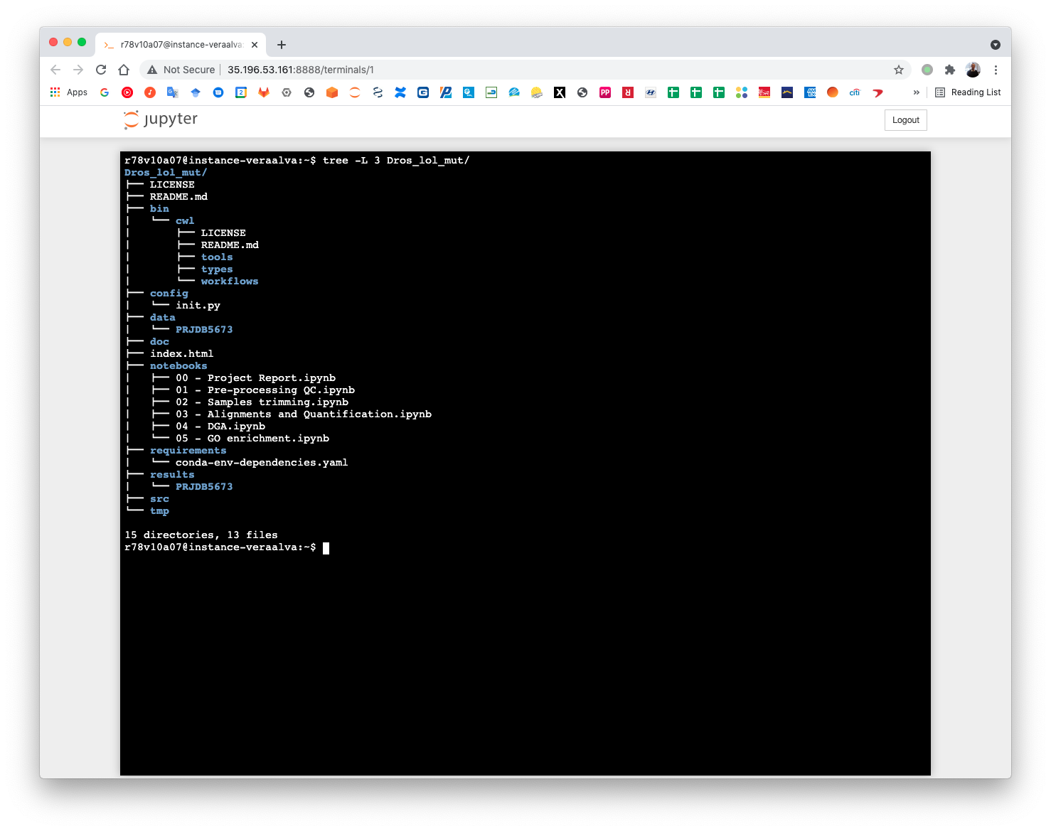
The project organizational data structure is:

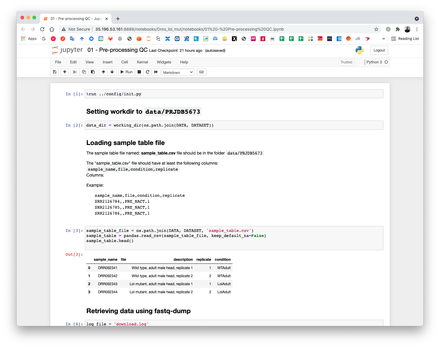
5.3. Pre-processing QC

The first notebook download the SRA data using the accessions defined in the sample sheet. Execute all cells until the Retrieving data using fastq-dump. This cell will submit the CWL workflow. Open a terminal to check that the fastq-dump command is working.

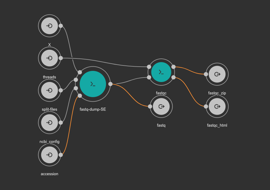
The CWL workflow for this step is: download_quality_control.cwl

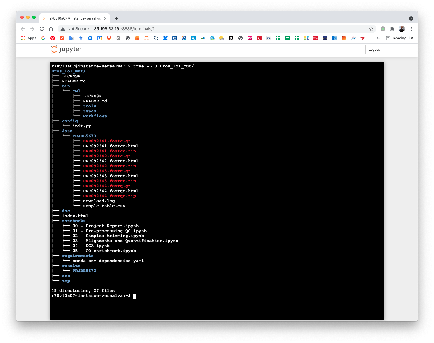
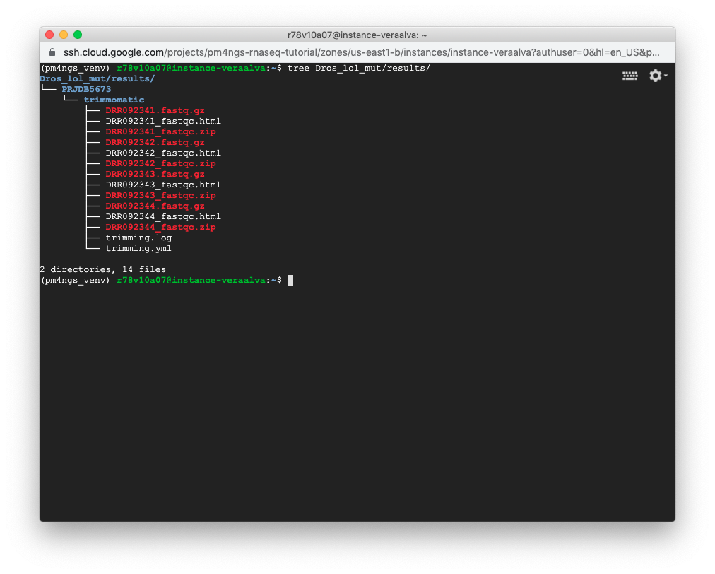
Once all cells are execute completely the fastq samples will be available at the data/PRJDB5673 directory. Run the tree command to visualize the data structure.

(pm4ngs_venv) r78v10a07@instance-veraalva:~$ tree -L 3 Dros_lol_mut/

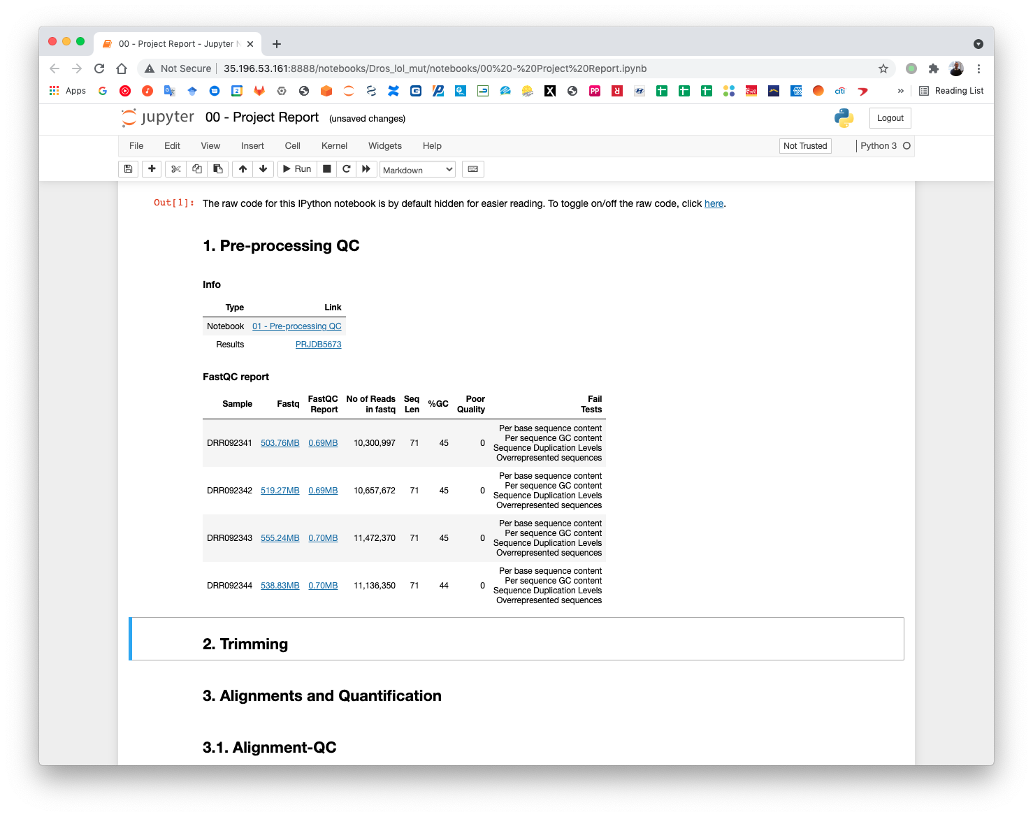
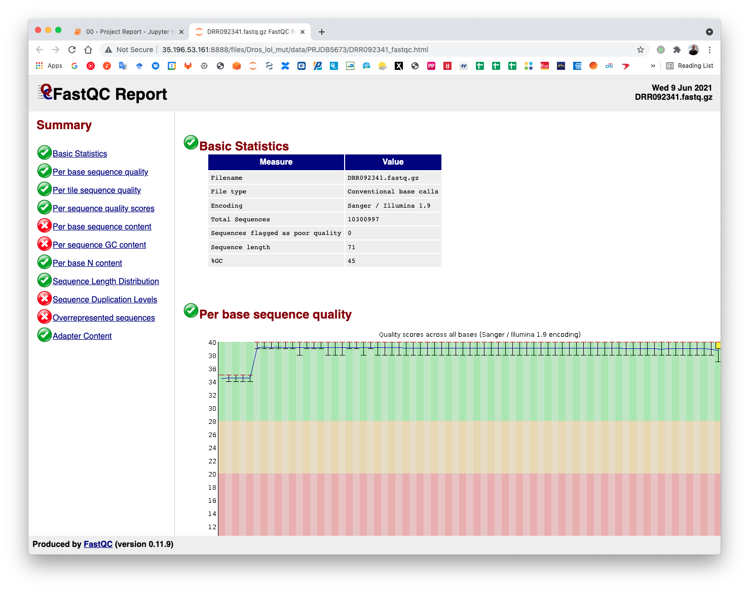
The pre-processing table is available in the 00 - Project Report notebook. The links in the table gives access to the FastQC reports for each sample. The reports are used to select the trimming parameters.

5.4. Samples trimming

Trimmomatic performs a variety of useful trimming tasks for illumina paired-end and single ended data.The selection of trimming steps and their associated parameters are supplied on the command line.

The current trimming steps are:

• ILLUMINACLIP: Cut adapter and other illumina-specific sequences from the read.

• SLIDINGWINDOW: Perform a sliding window trimming, cutting once the average quality within the window falls below a threshold.

• LEADING: Cut bases off the start of a read, if below a threshold quality

• TRAILING: Cut bases off the end of a read, if below a threshold quality

• CROP: Cut the read to a specified length

• HEADCROP: Cut the specified number of bases from the start of the read

• MINLEN: Drop the read if it is below a specified length

• TOPHRED33: Convert quality scores to Phred-33

• TOPHRED64: Convert quality scores to Phred-64

It works with FASTQ (using phred + 33 or phred + 64 quality scores, depending on the Illumina pipeline used), either uncompressed or gzipp'ed FASTQ. Use of gzip format is determined based on the .gz extension.

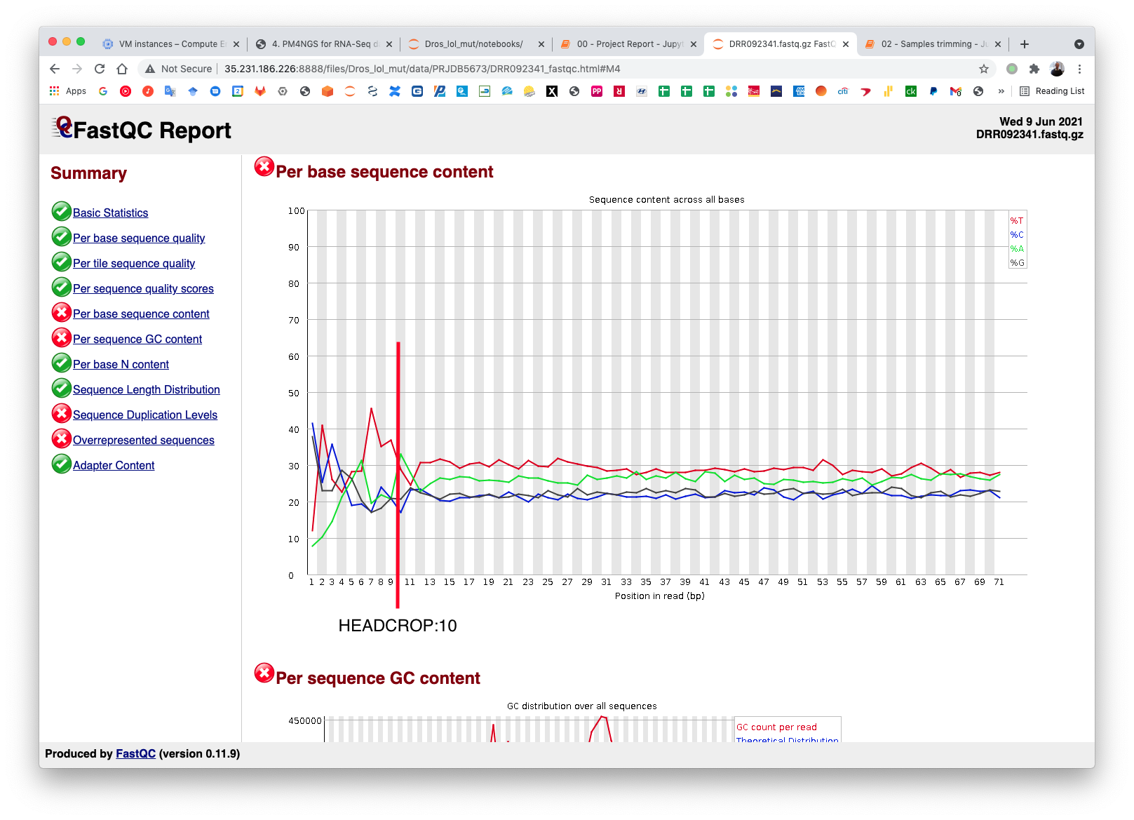
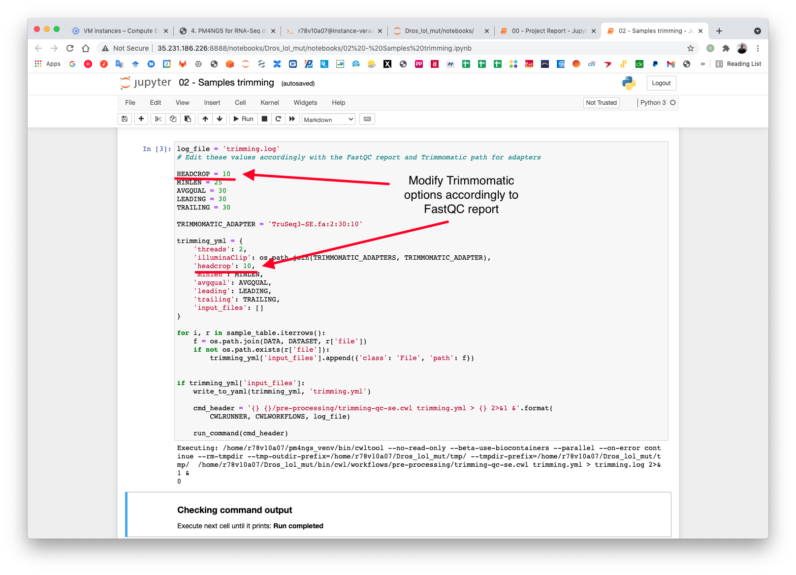
PM4NGS uses standard options for Trimmomatic but in this example we need to add HEADCROP:10 as it is shown in next figure:

The CWL workflow for this step is: trimming-qc-se.cwl

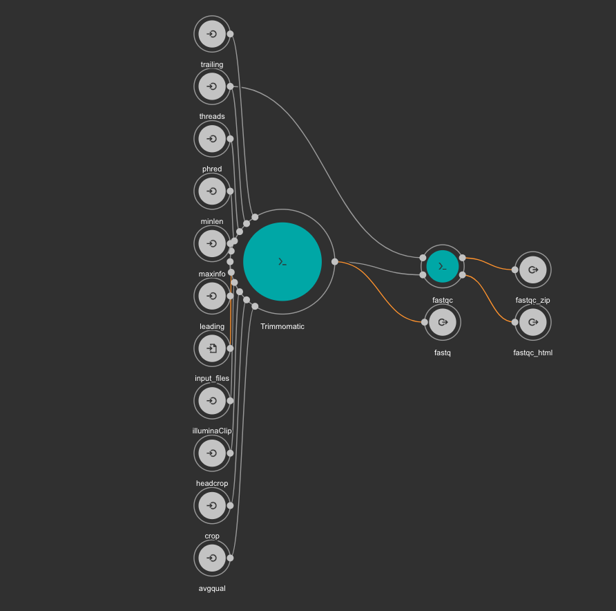
The result files for the trimming workflow are available at: results/PRJDB5673/trimmomatic

Updating the 00 - Project Report notebook.

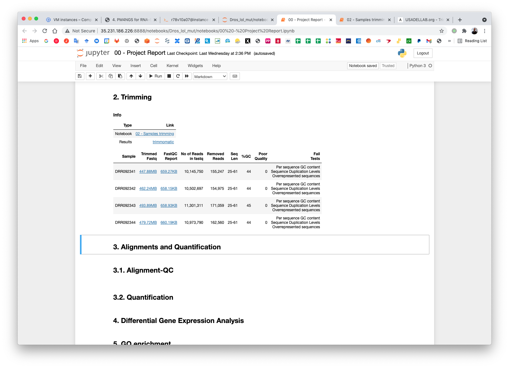
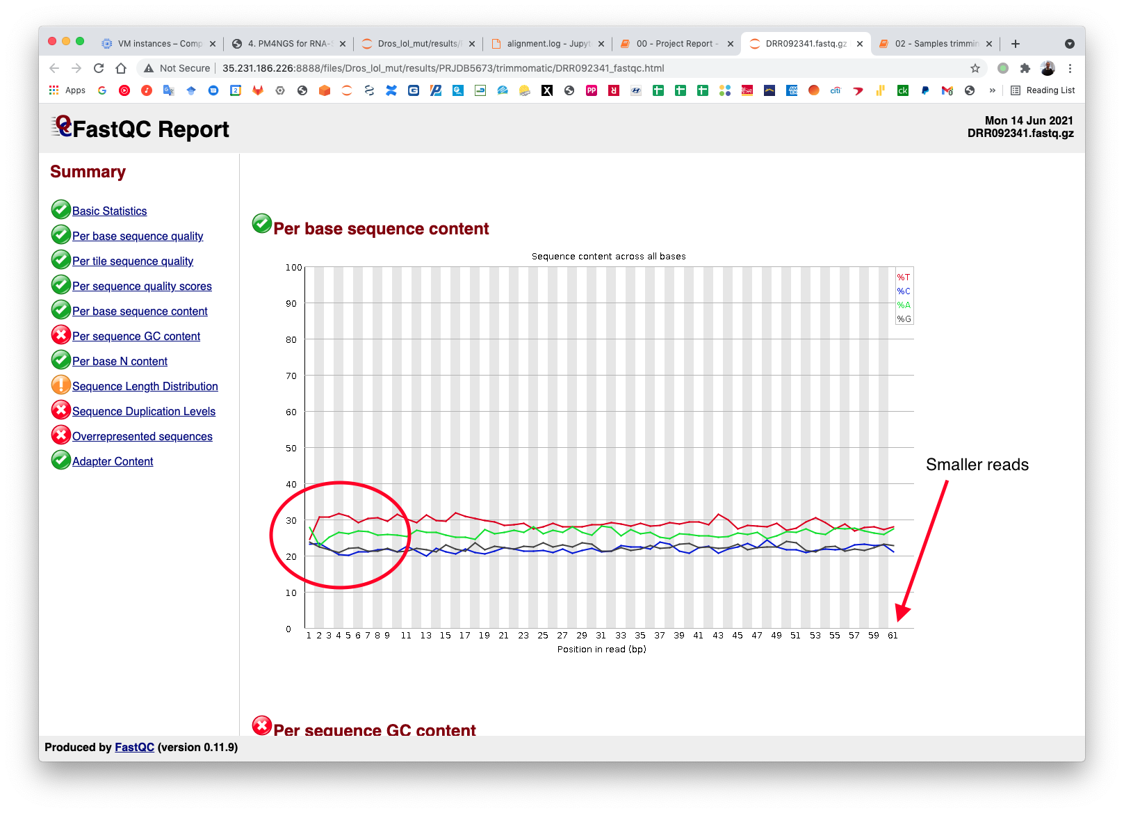
Check the FastQC reports to check if the trimming reduced the distortion in the first 10 bases.

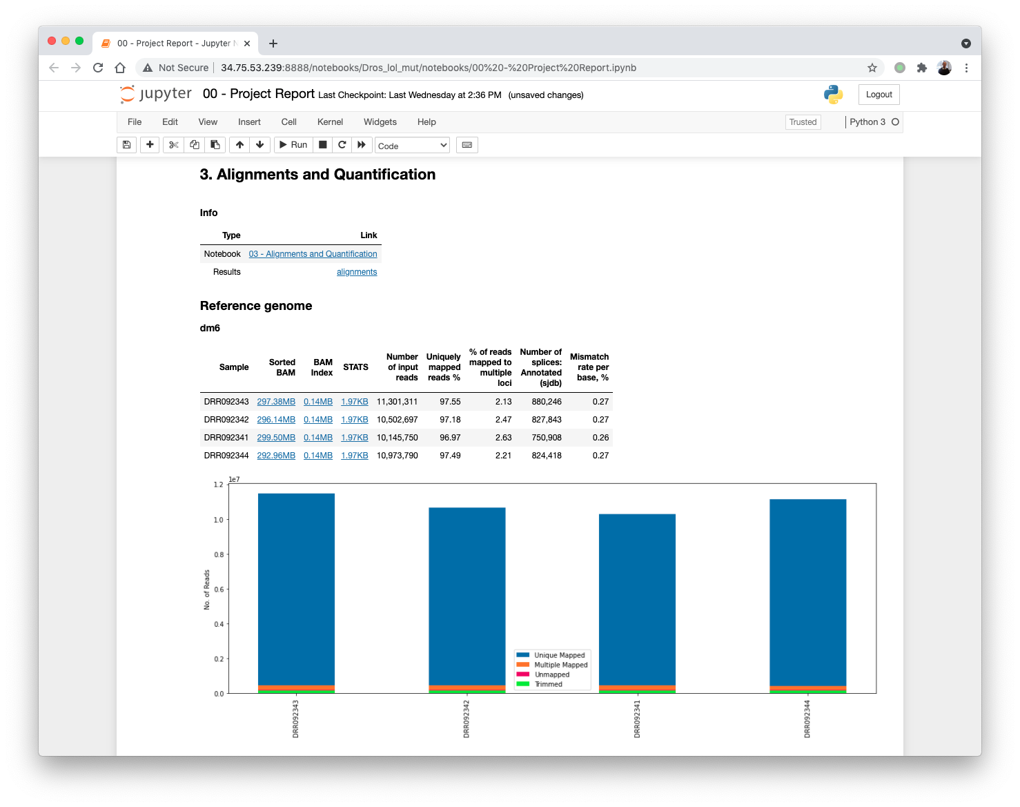
5.5. Alignment and Quantification

The alignment and quantification workflow uses STAR as aligner, Samtools for filtering and sorting BAM files, TPMCalculator for RNA-Seq quantification, RSeQC for post processing quality control and IGVtools for creating visualization files.

In this tutorial we are analysing Drosophila samples. Therefore, we need the Drosophila genome sequence and annotations. PM4NGS provides the dm6 genome pre-formatted for the alignment and quantification workflow. For a complete list of PM4NGS pre-formatted genomes see: https://pm4ngs.readthedocs.io/en/latest/pipelines/genomes.html

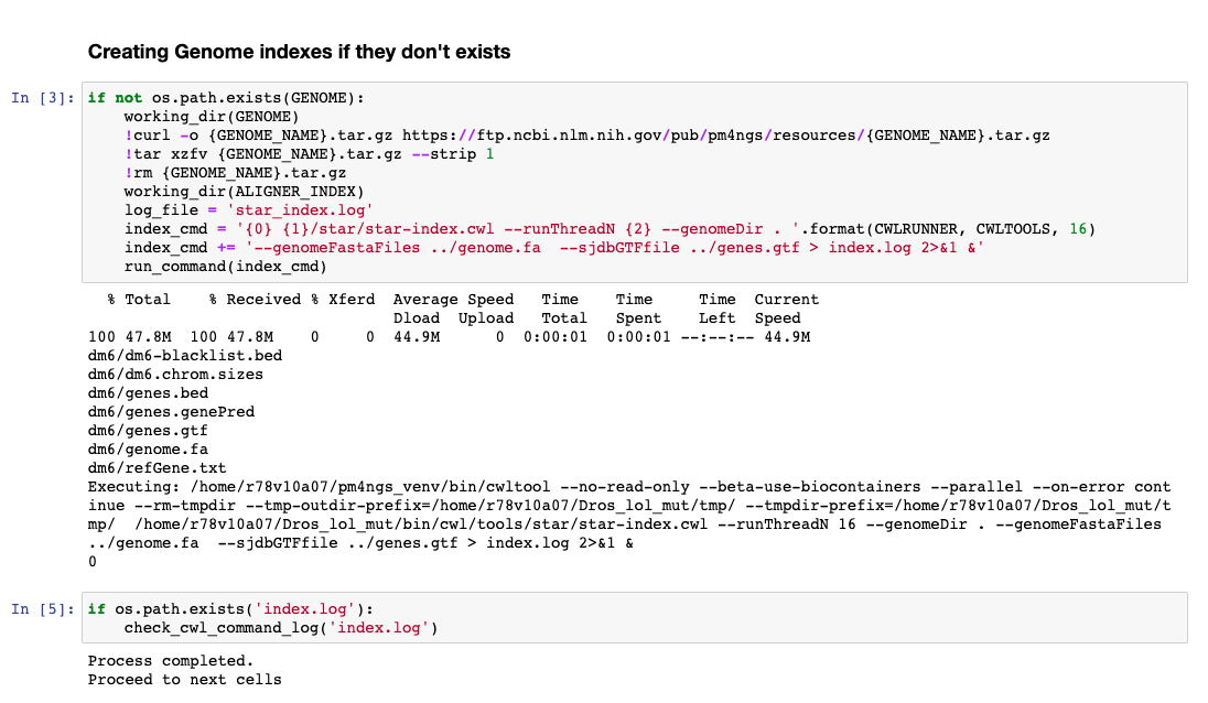
This workflow is the most time consuming part and require setting proper computer resources like number of cores and RAM. For this tutorial we need at least 64 GB of RAM and 16 cores. GCP machine type n1-standard-16 provides those resources.

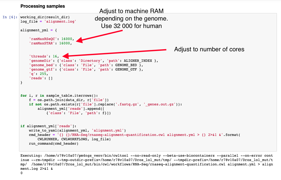
The CWL workflow for this step is: rnaseq-alignment-quantification.cwl

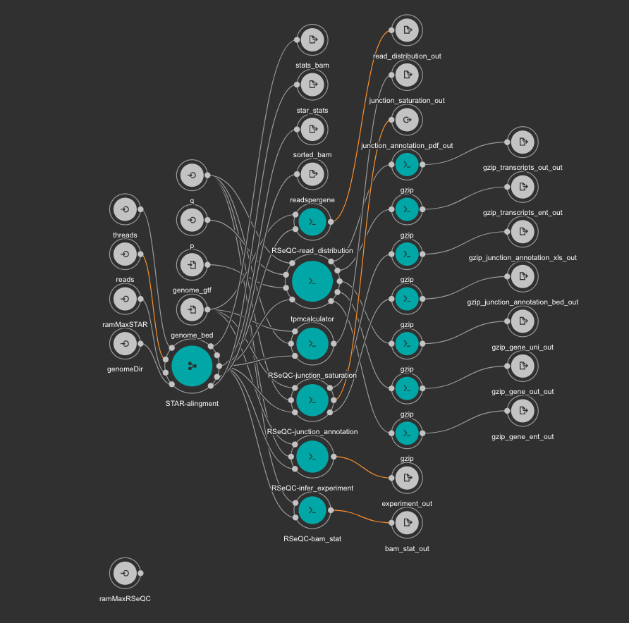
It is based in another workflow for the alignment: star-alignment.cwl

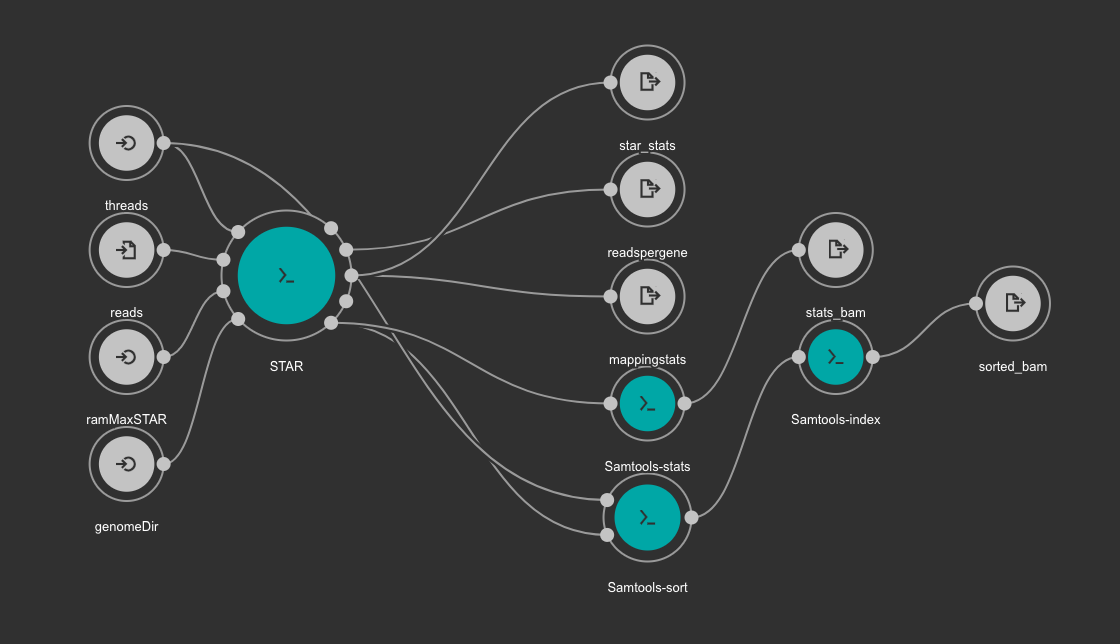
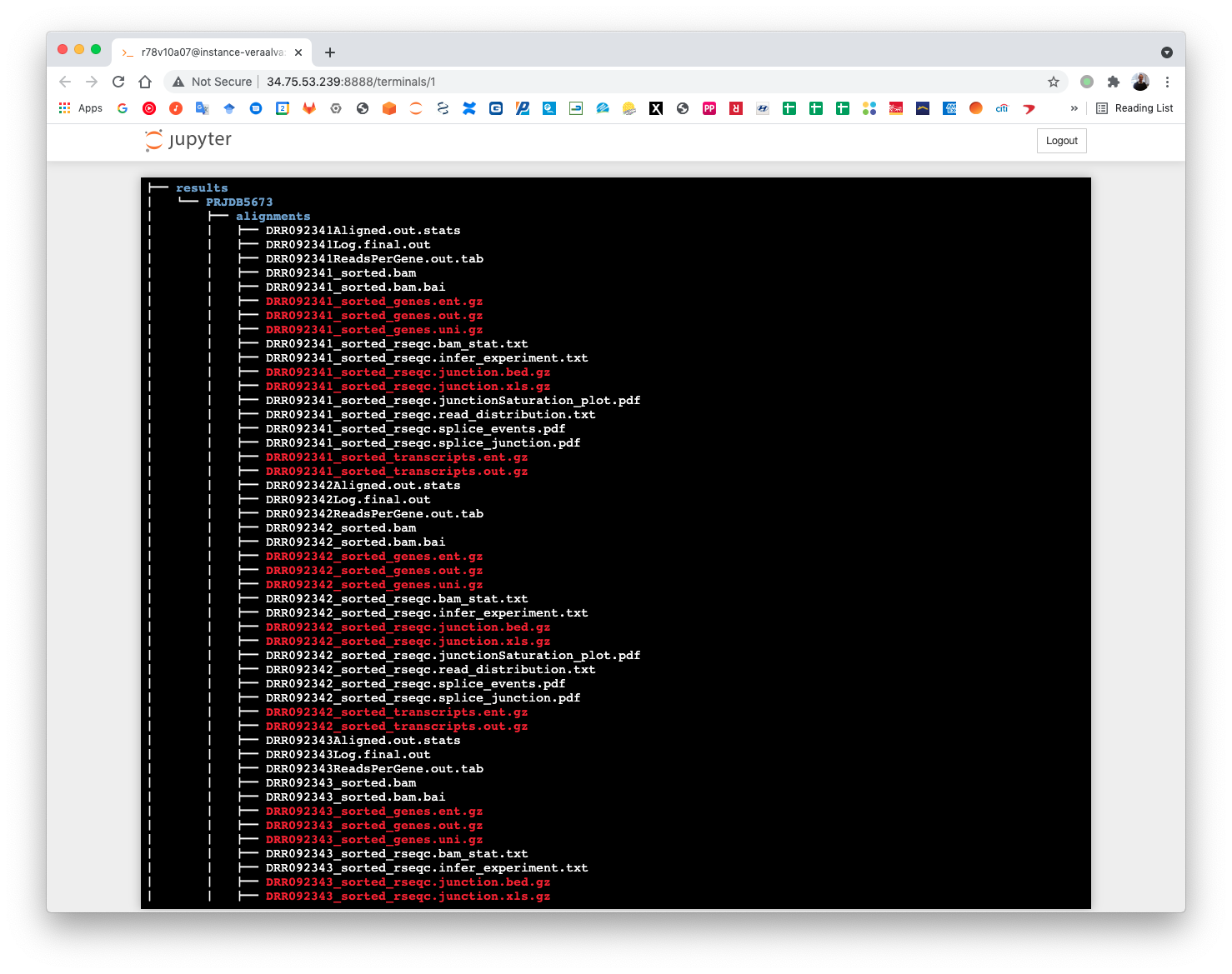
Once finished, the alignment and quantification workflow will create for each sample these files:

Note

STAR alignment stats

• DRR092341Aligned.out.stats

• DRR092341Log.final.out

• DRR092341ReadsPerGene.out.tab

Alignments files sorted from SAMtools

• DRR092341_sorted.bam

• DRR092341_sorted.bam.bai

Read counts and TPMs from TPMCalculator

• DRR092341_sorted_genes.ent.gz

• DRR092341_sorted_genes.out.gz

• DRR092341_sorted_genes.uni.gz

• DRR092341_sorted_transcripts.ent.gz

• DRR092341_sorted_transcripts.out.gz

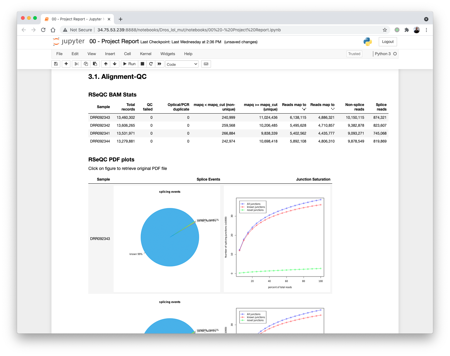
** Post-processing QC from RSeQC**

• DRR092341_sorted_rseqc.bam_stat.txt

• DRR092341_sorted_rseqc.infer_experiment.txt

• DRR092341_sorted_rseqc.junction.bed.gz

• DRR092341_sorted_rseqc.junction.xls.gz

• DRR092341_sorted_rseqc.junctionSaturation_plot.pdf

• DRR092341_sorted_rseqc.read_distribution.txt

• DRR092341_sorted_rseqc.splice_events.pdf

• DRR092341_sorted_rseqc.splice_junction.pdf

Updating the 00 - Project Report notebook.

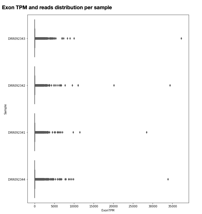
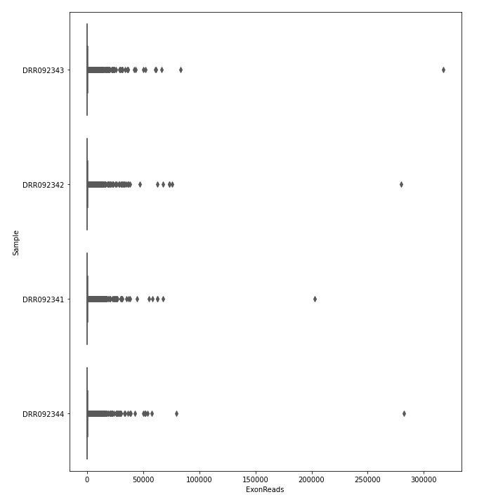
The quantification values read counts and TPM are shown in a boxplot for easy comparison.

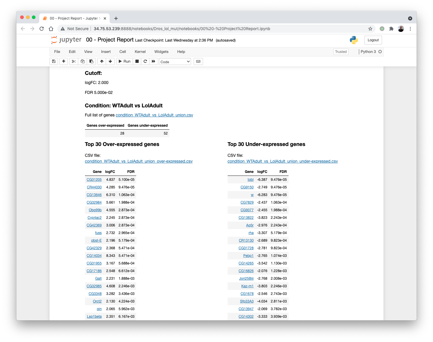
5.6. Differential Gene Expression Analysis

The DGE analysis is executed in the 04 - DGA notebook. The workflow uses DESeq2 and EdgeR for the identification of differentially expressed genes. R scripts are available at deseq2-2conditions.cwl and edgeR-2conditions.cwl.

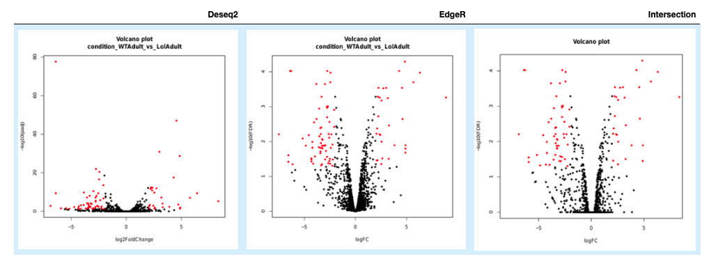
In our approach, genes are designated as differentially expressed if they are identified by DESeq2 and EdgeR. Those genes are shown under the Intersection results.

results/PRJDB5673/dga/
├── WTAdult_vs_LolAdult_deseq2_dga.log
├── WTAdult_vs_LolAdult_edge_dga.log
├── WTAdult_vs_LolAdult_heatmap_union.log
├── WTAdult_vs_LolAdult_volcano_union.log
├── condition_WTAdult_vs_LolAdult_deseq2.csv
├── condition_WTAdult_vs_LolAdult_deseq2_correlation_heatmap.pdf
├── condition_WTAdult_vs_LolAdult_deseq2_expression_heatmap.pdf
├── condition_WTAdult_vs_LolAdult_deseq2_pca.csv
├── condition_WTAdult_vs_LolAdult_deseq2_pca.pdf
├── condition_WTAdult_vs_LolAdult_deseq2_volcano.pdf
├── condition_WTAdult_vs_LolAdult_edgeR.csv
├── condition_WTAdult_vs_LolAdult_edgeR_correlation_heatmap.pdf
├── condition_WTAdult_vs_LolAdult_edgeR_expression_heatmap.pdf
├── condition_WTAdult_vs_LolAdult_edgeR_pca.csv
├── condition_WTAdult_vs_LolAdult_edgeR_pca.pdf
├── condition_WTAdult_vs_LolAdult_edgeR_volcano.pdf
├── condition_WTAdult_vs_LolAdult_intersection.csv
├── condition_WTAdult_vs_LolAdult_intersection_correlation_heatmap.pdf
├── condition_WTAdult_vs_LolAdult_intersection_expression_heatmap.pdf
├── condition_WTAdult_vs_LolAdult_intersection_over-expressed.csv
├── condition_WTAdult_vs_LolAdult_intersection_pca.pdf
├── condition_WTAdult_vs_LolAdult_intersection_under-expressed.csv
└── condition_WTAdult_vs_LolAdult_intersection_volcano.pdf

0 directories, 23 files

Updating the 00 - Project Report notebook.

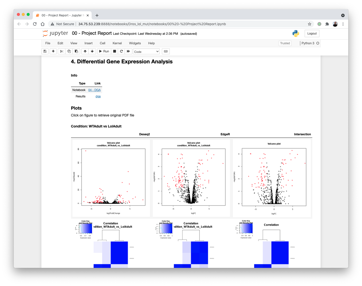
DGE plots are automatically generated.

5.6.1. Volcano Plots

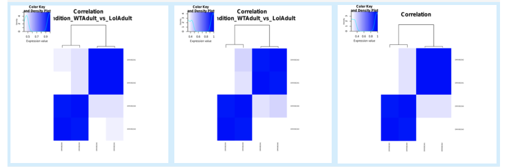
5.6.2. Sample correlation

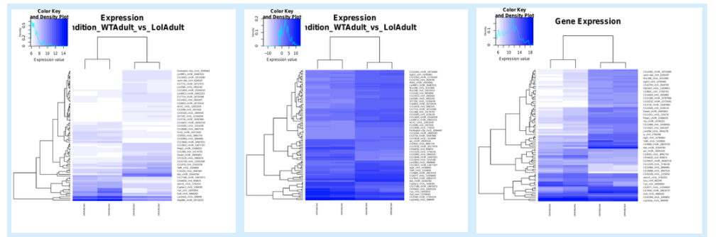
5.6.3. Expression correlation

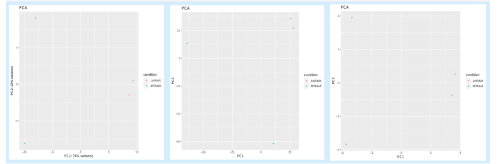
5.6.4. PCA plots

5.6.5. List of differentially expressed genes

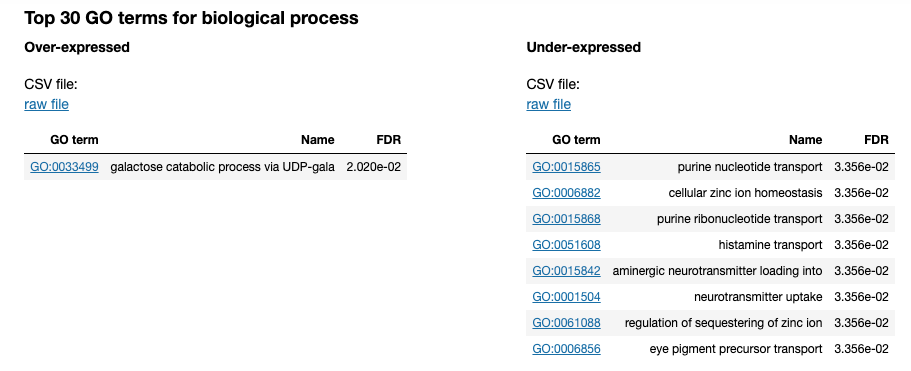
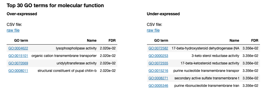
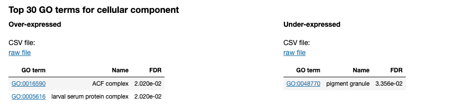
5.7. Gene Ontology Enrichment

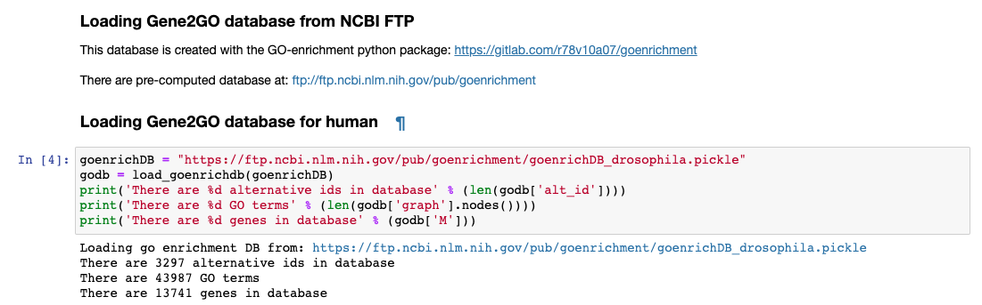
Gene Ontoogy enrichment analysis is executed with an in-house developed python package named goenrichment. This tool creates a database by integrating information from Gene Ontology, NCBI Gene using the files gene_info and gene2go. Read more in the package web page to create a database for another organism.

Available databases can be downloaded from https://ftp.ncbi.nlm.nih.gov/pub/goenrichment/

Next image shows the pre-defined code in PM4NGS for downloading the GO enrichment database for Drosophila. Current version of the database contains 43 987 GO terms cros-referenced to 13 741 genes.

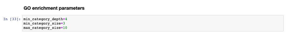
The GO enrichment tool uses three parameters to identify differential GO terms between the two conditions.

Note

min_category_depth

Min GO term graph depth to include in the report. Default: 4

min_category_size

Min number of gene in a GO term to include in the report. Default: 3

max_category_size

Max number of gene in a GO term to include in the report. Default: 500 This 500 is good for very well annotated organism as human or mouse.

In the case of Drosophila use 10 to get relevant results.

In the Jupyter Notebook change the values to

Updating the 00 - Project Report notebook.

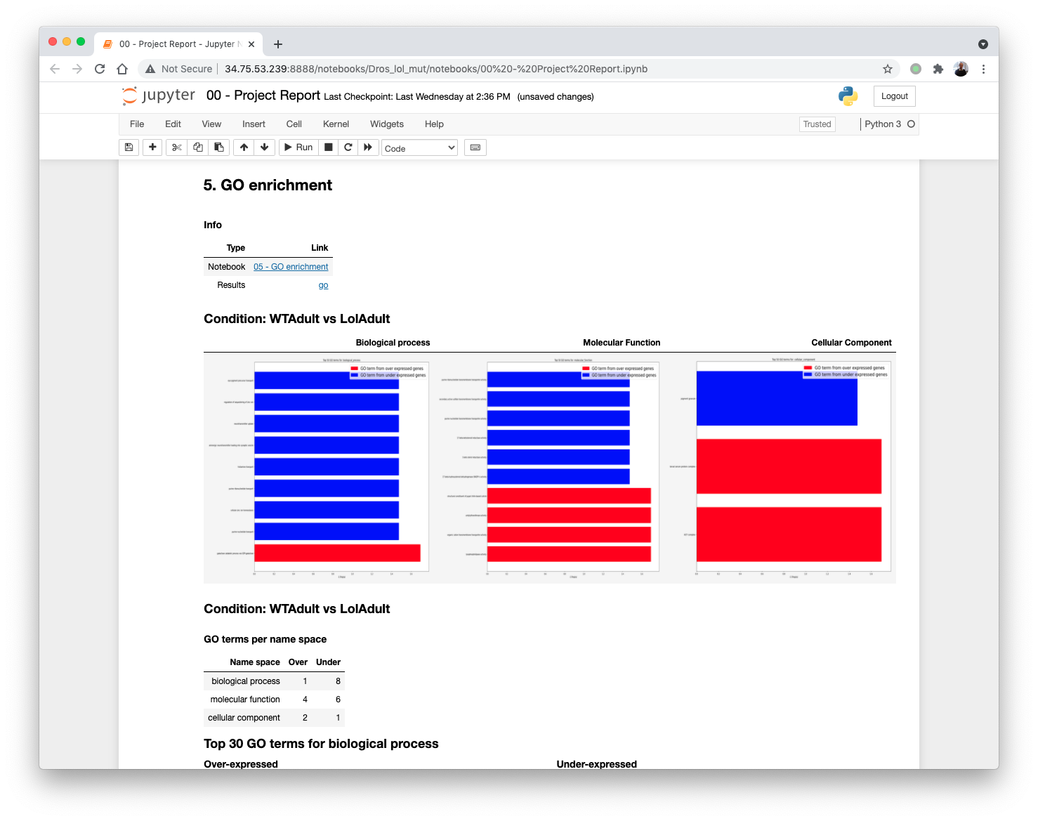
The list of differential GO terms are available in the tables per GO name space.